Pushing the boundaries of actuators-to-task kinematic inversion: from fully actuated to underactuated (soft) robots

Della Santina, Cosimo

The International Journal of Robotics Research · in press

Pushing the boundaries of actuators-to-task kinematic inversion: from fully actuated to underactuated (soft) robots

Inverse kinematics for robots that cannot hold every pose.

Conventional closed-loop inverse kinematics assumes that actuators can maintain arbitrary robot configurations. We extend this approach to underactuated robots, such as soft arms, tendon-driven hands, and balancing humanoids, by introducing two algorithms that solve arbitrary tasks by computing configurations the robot can physically maintain.

Cosimo Della Santina
Faculty of Mechanical Engineering, Delft University of Technology

Plain inverse kinematics reaches the target $\bar x$ with a shape the arm cannot hold: gravity and springs move it along the direction the tendon leaves free. The solution has to lie on the set $\mathcal{E}$ of shapes the arm can hold.

Citation

@article{dellasantina2026underactuated,
  title   = {Pushing the boundaries of actuators-to-task kinematic inversion:
             from fully actuated to underactuated (soft) robots},
  author  = {Della Santina, Cosimo},
  journal = {The International Journal of Robotics Research},
  year    = {2026},
  note    = {In press; volume, pages and DOI to follow}
}

Fewer actuators than degrees of freedom

The robots we have in mind

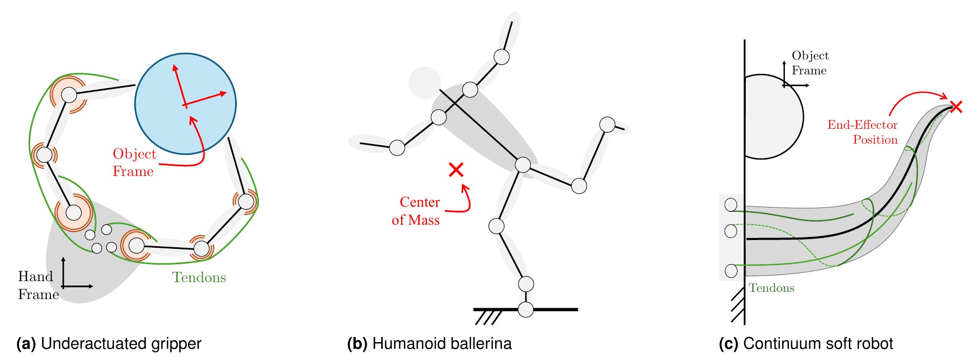
Three underactuated robots: a two-finger gripper driven by four tendons holding a ball, a humanoid balancing on one tip while regulating its centre of mass, and a tendon-driven continuum soft robot reaching an object with its tip — (a) A two-finger gripper driven by four tendons manipulates a ball: 7 degrees of freedom, 4 actuators, a 3-dimensional task. (b) A humanoid balancing on its tip regulates its centre of mass: 11 degrees of freedom, 10 actuators, a 2-dimensional task. (c) A continuum soft robot driven by three tendons positions its tip: infinitely many degrees of freedom, 3 actuators, a 3-dimensional task. In all three, inverse kinematics must return a configuration the robot can hold.

Explainer 1 · 1.5 min

The problem

With a motor at every joint, inverse kinematics is essentially a geometric problem: any configuration that reaches the target can, in principle, be maintained by the motors. Replace two motors with a single tendon, however, and one direction of motion remains unactuated. Along this direction, the equilibrium is determined by gravity and elastic forces. Consequently, most configurations that reach the target can no longer be maintained. The configurations that the robot can hold form an equilibrium manifold $\mathcal{E}$, and any valid inverse-kinematics solution must lie within it.

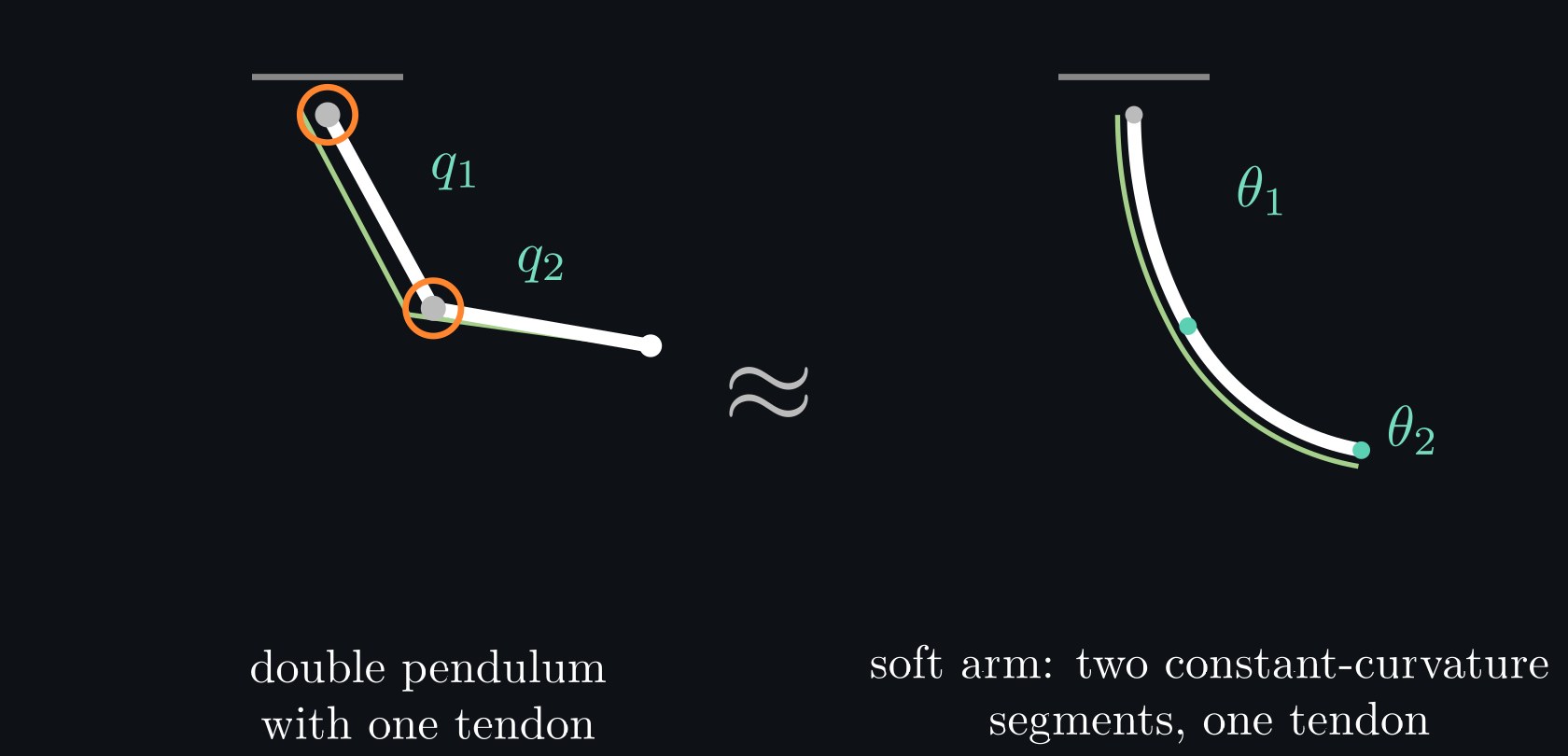
From the fully actuated arm to a tendon-driven double pendulum. The goal: a loop that brings the tip to the target and the shape onto $\mathcal{E}$.

What the paper contributes

Inverse kinematics on configurations the robot can hold

A general formulation

We extend closed-loop inverse kinematics to underactuated mechanical systems by restricting solutions to the set of configurations the robot can maintain in static equilibrium. Classical IK is recovered as the fully actuated special case, while actuator-space inversion in soft robotics corresponds to a flat equilibrium set.

Algorithm 1

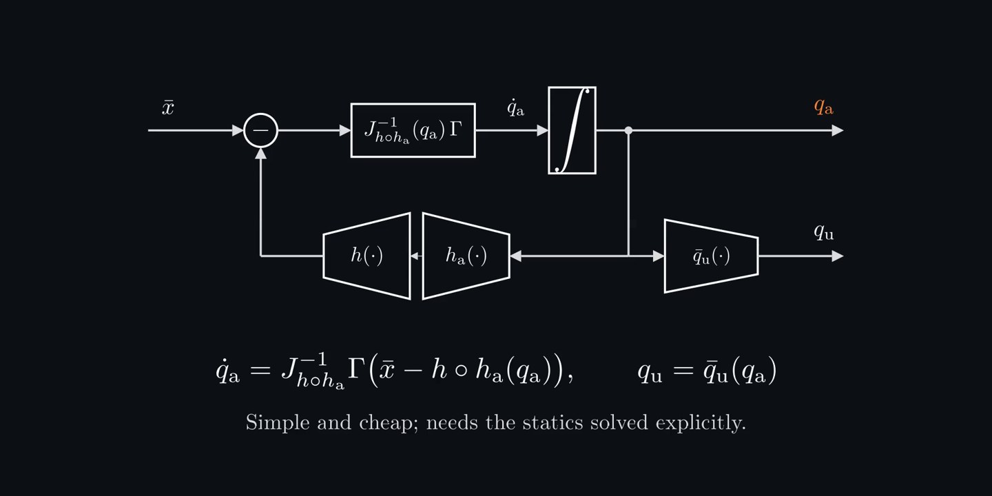
When the passive coordinates can be determined by solving the statics in advance, we formulate CLIK directly on the equilibrium set and establish conditions for exponential convergence.

Algorithm 2

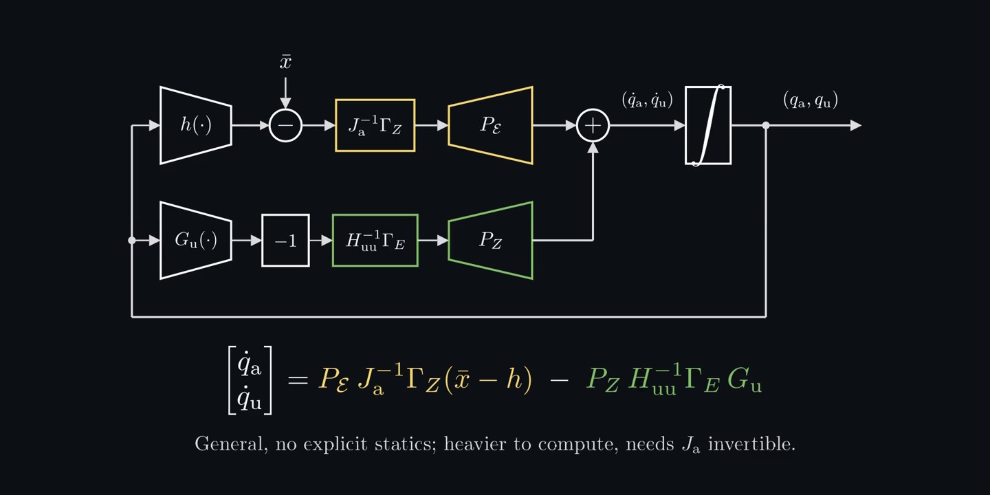
We express static equilibrium as a holonomic constraint and incorporate it into the control loop as an additional task, following constrained CLIK. This avoids explicitly solving the statics while retaining formal convergence conditions.

Explainers 2 and 3

Two algorithms to stay on $\mathcal{E}$

Notation used below

$q$: configuration of the robot: joint angles, curvatures, shape parameters ($n$ of them)
$q_{\mathrm a}$: actuated coordinates, set directly by the actuators: motor angles, tendon lengths ($m < n$ of them). In the double pendulum, $q_{\mathrm a}$ is the tendon length, a weighted sum of the two joint angles
$q_{\mathrm u}$: unactuated coordinates: what still moves when the actuators are locked. In the double pendulum, $q_{\mathrm u}$ is the joint motion that keeps the tendon length fixed
$x = h(q)$, $\bar x$: task variable (for example the tip position) and its target
$G(q)$, $G_{\mathrm u}$: potential forces (gravity, springs) and their part along $q_{\mathrm u}$. We change coordinates from $q$ to $(q_{\mathrm a}, q_{\mathrm u})$ so that the actuators push only on $q_{\mathrm a}$, so nothing balances $G_{\mathrm u}$: with the actuators locked, the robot stays still only where $G_{\mathrm u} = 0$. Solving $G_{\mathrm u} = 0$ is what we call solving the statics
$\mathcal{E}$: configurations the robot can hold, that is static equilibria: $G_{\mathrm u}(q) = 0$. $\mathcal{E}$ also contains unstable equilibria. $H_{\mathrm{uu}} = \partial G_{\mathrm u}/\partial q_{\mathrm u}$ is the stiffness the robot feels along $q_{\mathrm u}$ with the actuators locked, and the equilibrium is stable when it is positive ($H_{\mathrm{uu}} \succ 0$). Neither algorithm checks this, and a collocated controller that feeds back only $q_{\mathrm a}$ cannot stabilize the others; that takes feedback on $q_{\mathrm u}$ too (see the dancer, Unstable target)

More symbols: Jacobians, Hessian blocks, projectors, gains

$\bar q_{\mathrm u}(q_{\mathrm a})$, $h_{\mathrm a}$: the held $q_{\mathrm u}$ for given actuators, and the resulting configuration (Algorithm 1). The actuators-to-task map is $h\circ h_{\mathrm a}$
$J_{\mathrm a}, J_{\mathrm u}$: task Jacobians with respect to $q_{\mathrm a}$ and $q_{\mathrm u}$
$H_{\mathrm{ua}}, H_{\mathrm{uu}}$: derivatives of $G_{\mathrm u}$ with respect to $q_{\mathrm a}$ and $q_{\mathrm u}$
$P_{\mathcal E}, P_{\mathcal Z}$: projectors: $P_{\mathcal E}$ turns a task correction into a motion that keeps $G_{\mathrm u}$ unchanged, $P_{\mathcal Z}$ turns a statics correction into a motion that keeps $h$ unchanged, both to first order (Algorithm 2)
$\Gamma, \Gamma_{\mathcal Z}, \Gamma_{\mathcal E}$: positive-definite gains
dimensions: the formulas assume a task with as many dimensions as actuators, $m$. With fewer (Fig. 1a, b and the dancer below), inverses become pseudoinverses

A fuller, robot-oriented version is in the practitioner's guide.

Algorithm 1 · statics solved beforehand

Fix the actuators and the robot settles in a held configuration. Where $H_{\mathrm{uu}}$ is invertible, the statics define a local branch $q_{\mathrm u} = \bar q_{\mathrm u}(q_{\mathrm a})$: pick a stable one and solve it beforehand. The result is a map from actuators to task, defined on held configurations only, and classic closed-loop IK runs on it with Jacobian $J = J_{\mathrm a} - J_{\mathrm u} H_{\mathrm{uu}}^{-1} H_{\mathrm{ua}}$: differentiating $G_{\mathrm u}(q_{\mathrm a}, \bar q_{\mathrm u}(q_{\mathrm a})) = 0$ gives $\partial \bar q_{\mathrm u}/\partial q_{\mathrm a} = -H_{\mathrm{uu}}^{-1}H_{\mathrm{ua}}$, and the chain rule does the rest.

$\dot q_{\mathrm a} = J_{h\circ h_{\mathrm a}}^{-1}\,\Gamma\,\big(\bar x - h\circ h_{\mathrm a}(q_{\mathrm a})\big)$

Block diagram: the task error is mapped through the inverse Jacobian of the actuators-to-task map and integrated into actuator coordinates; the passive coordinates follow from the statics

Needs: an explicit solution of the statics, $\bar q_{\mathrm u}(q_{\mathrm a})$
Gives: a light loop with one coordinate per actuator; every intermediate reference lies on $\mathcal{E}$

Watch the full explainer (3 min, includes a side note for soft roboticists)

Algorithm 2 · statics solved online

When $G_{\mathrm u}=0$ cannot be solved for $q_{\mathrm u}$ in advance, the loop solves it online. It asks both the task error and $G_{\mathrm u}$ to decay exponentially, so the statics hold asymptotically; at each step that gives a linear system in $(\dot q_{\mathrm a}, \dot q_{\mathrm u})$:

$J_{\mathrm a}\dot q_{\mathrm a} + J_{\mathrm u}\dot q_{\mathrm u} = \Gamma_{\mathcal Z}(\bar x - h)$
$H_{\mathrm{ua}}\dot q_{\mathrm a} + H_{\mathrm{uu}}\dot q_{\mathrm u} = -\Gamma_{\mathcal E} G_{\mathrm u}$

The projectors $P_{\mathcal E}$, $P_{\mathcal Z}$ write out its solution. Where $\mathcal{E}$ meets the target set in several points, the loop reaches one of them, depending on where it starts.

$(\dot q_{\mathrm a}, \dot q_{\mathrm u}) = P_{\mathcal E} J_{\mathrm a}^{-1}\Gamma_{\mathcal Z}(\bar x - h) - P_{\mathcal Z} H_{\mathrm{uu}}^{-1}\Gamma_{\mathcal E} G_{\mathrm u}$

$Block diagram with two parallel paths: a task path through the inverse actuated Jacobian and the lift P_E, a feasibility path through the inverse Hessian block and the lift P_{\mathcal Z}, summed and integrated$

Needs: gradients of $h$ and $G_{\mathrm u}$; $J_{\mathrm a}$, $H_{\mathrm{uu}}$ and $I - J_{\mathrm a}^{-1}J_{\mathrm u}H_{\mathrm{uu}}^{-1}H_{\mathrm{ua}}$ invertible along the way (the last one: the actuators still move the task along $\mathcal{E}$)
Gives: starts anywhere these inverses stay well defined, also off $\mathcal{E}$; no case-by-case derivation; heavier per step

Watch the full explainer (2 min)

Interactive · runs in your browser

Try it: the tendon-driven arm

This is the running example of the paper: a double pendulum with one tendon, joint springs and gravity. The task is the horizontal position of the tip, so the shapes that reach it, $h(q) = \bar x$, form a curve; thin dashed lines join shapes with the same tendon length. Pick a method and press Run. Drag the target on the left, or click in the configuration space on the right to choose where the loop starts.

Run plain IK: the arm reaches the target, then sags once released, because that shape is not an equilibrium.
Run Algorithm 1: every reference along the way lies on $\mathcal{E}$.
Click far from $\mathcal{E}$ in the configuration space, then run Algorithm 2: both errors decay in the plot.
Set gravity to zero: $\mathcal{E}$ becomes a straight line.
Run Algorithm 1, then drag the target: the solution slides along $\mathcal{E}$.

Show where the arm settles

The arm. Grey ghost: where it settles if the tendon stays at its current length.

Configuration space $(q_1, q_2)$. Click, or focus and use the arrow keys, to choose the start.

Neither held nor at the target task error 0 statics residual $|G_{\mathrm u}|$ 0

Target $\bar x$ 1.20

Gravity $g$ 9.8

Spring, joint 1 0

Spring, joint 2 10

Tendon routing $\theta$ 23°

A double pendulum with one tendon next to a soft arm made of two constant-curvature segments with one tendon

Read it as a soft arm. The running example is close to a soft arm made of two constant-curvature segments driven by one tendon. The joint angles $q_1, q_2$ become the bending angles $\theta_1, \theta_2$ of the segments, the joint springs their bending stiffness, and the tendon runs along both segments, so it sets $q_{\mathrm a} \propto \theta_1 + \theta_2$ and leaves $\theta_1 - \theta_2$ free. The pseudocode of both algorithms carries over unchanged; the walkthrough videos in the practitioner's guide end with this mapping.

Interactive · drag to rotate

Three joints, two tendons: $\mathcal{E}$ becomes a surface

With three joints and two tendons, the configuration space is three-dimensional and $\mathcal{E}$ is a two-dimensional sheet inside it. The view uses actuation coordinates: two directions set by the tendons, one direction they do not fix. Launch trajectories of either strategy and watch where they go.

Show the flat sheet (fully actuated picture)

The arm, one colour per trajectory.

sheet $\mathcal{E}$, coloured by $q_{\mathrm u}$ lines of constant actuation configurations with $h(q)=\bar x$ held solution dashed: from an Algorithm 2 start down to the sheet, for depth only

Gravity $g$ 9.8

The $q_{\mathrm u}$ axis is stretched so the shape of the sheet is visible; the stretch also exaggerates how far Algorithm 2 paths leave the sheet. Set gravity to zero and switch on the flat sheet: they coincide.

Side note

If you work in soft robotics

You may recognize the familiar picture of continuum robotics: actuator, configuration, and task spaces, with an actuation model connecting the first two. In this simplified representation, all three spaces have the same dimension, and the actuators fully determine the robot’s configuration.

In reality, the configuration space is much larger. The configurations the robot can maintain in equilibrium form a lower-dimensional set $\mathcal{E}$, whose dimension matches the number of actuators. The mapping from actuation to task space is defined on $\mathcal{E}$.

Interestingly, when gravity is neglected, elasticity is linear, stiffness is uniform within each actuated section, and the rest shape is straight, $\mathcal{E}$ becomes exactly the flat surface assumed by the familiar representation. This helps explain why the fully actuated approximation has worked so well in practice.

Results

Simulations: a soft arm and a balancing dancer

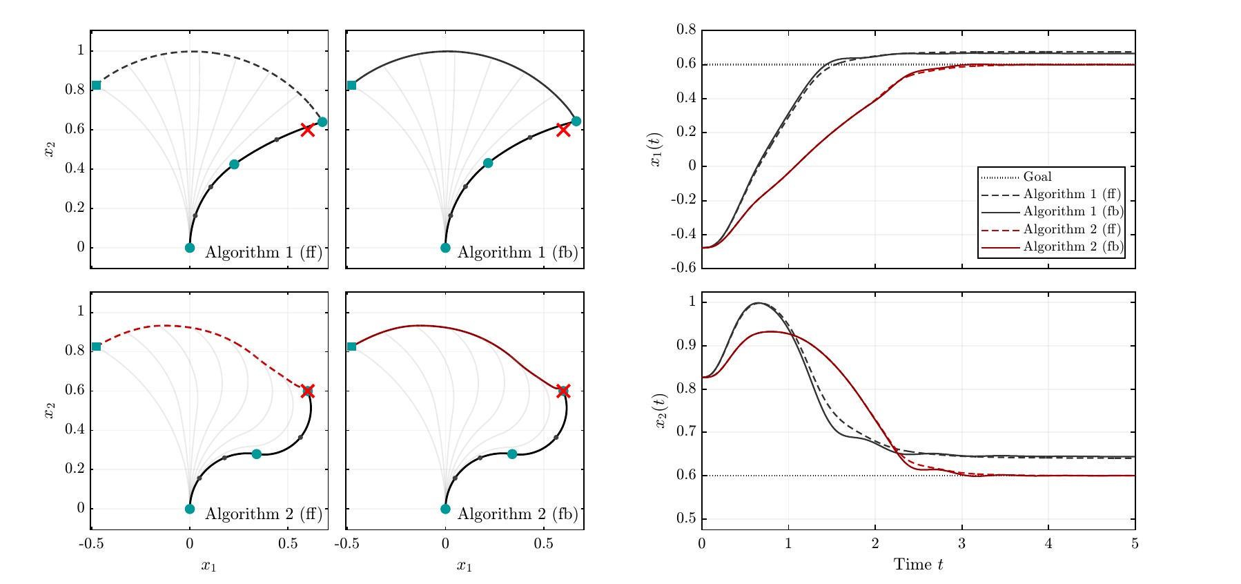
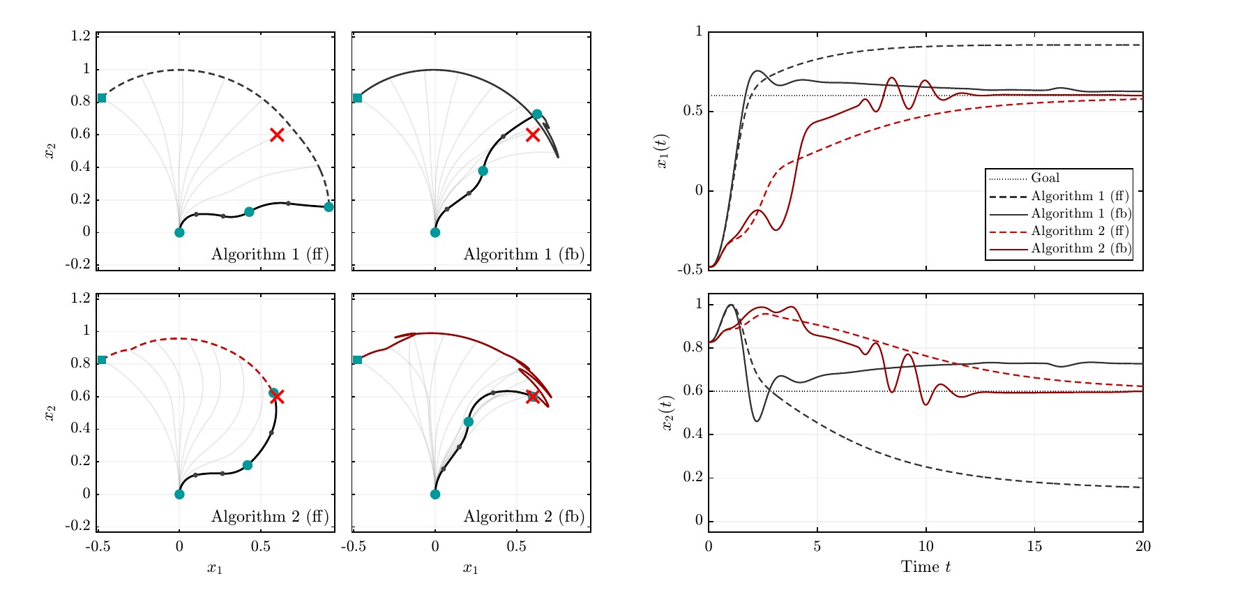
Takeaway. Algorithm 2 approaches the target in every soft-arm experiment. For Algorithm 1, accuracy depends on the quality of the statics model: improving the model or introducing feedback reduces the tracking error. On the dancer, both algorithms track the reference, although a 20% model error introduces steady-state offsets. Unstable target configurations, instead, cannot be maintained.

We test both algorithms on both systems, in feedforward (ff) and feedback (fb) modes. In feedforward mode, the algorithm computes the task error using its own predicted state $\bar q$; in feedback mode, it uses the measured robot configuration $q$. A low-level controller tracks the commanded actuated coordinates $\bar q_{\mathrm a}$, while the passive coordinates $q_{\mathrm u}$ evolve according to the robot’s mechanics.

For Algorithm 1, we deliberately use a statics model that neglects gravity, to illustrate the consequences of this approximation, together with a Jacobian-transpose update $\dot q_{\mathrm a} = J^\top \Gamma e$.

Videos play in real time. Click to pause.

A planar continuum arm: stiff and soft

We consider a planar soft arm represented by five constant-curvature segments and driven by two actuated sections. Its configuration $q$ consists of five curvature coordinates, two actuated ($q_{\mathrm a}$) and three passive ($q_{\mathrm u}$), while the task $x$ is the two-dimensional position of the tip.

Top: robot motion under the four algorithm variants. The red cross marks the target, and the teal dots indicate the section endpoints.
Bottom (wide screens only): evolution of the tip coordinates over time.

The corresponding figures of the paper

Stiff arm: tip trajectories and task coordinates over time for Algorithms 1 and 2, feedforward and feedback — Stiff arm (Fig. 18). Left: tip trajectories and final shapes; right: task coordinates over time.

Soft arm: tip trajectories and task coordinates over time for Algorithms 1 and 2 — Soft arm (Fig. 19).

A dancer on an elastic pointe

A simple version of the balancing system of Fig. 1(b): a planar dancer standing on one pointe, modelled as a passive torsional spring with a damper. The hips and the shoulder are actuated; the task is the position of the centre of mass. Three actuators and a two-dimensional task make the inversion redundant: Algorithm 1 uses a pseudoinverse, Algorithm 2 a non-square generalization of its projectors (see the code).

Practitioner's guide

Using the algorithms on your robot

1. Match the math to your robot

$q$: the full configuration: joint angles, curvatures, shape parameters
$q_{\mathrm a}$: actuated coordinates: motor angles, tendon lengths, chamber volumes
$q_{\mathrm u}$: what still moves if you block the actuators: passive joints, curvature differences within a segment
$c(q)$: the map $q \mapsto (q_{\mathrm a}, q_{\mathrm u})$; in practice choose $q_{\mathrm a}$ from the actuators and add enough $q_{\mathrm u}$ to fix the shape
$x = h(q)$: the task: tip position, pose, centre of mass, contact point
$G(q)$: potential forces (elastic, gravitational): what remains of the dynamics after removing all terms in $\ddot q$, $\dot q$ and $\tau$
$G_{\mathrm u}$: the part of $G$ along $q_{\mathrm u}$: forces the actuators cannot counteract. Held configurations satisfy $G_{\mathrm u}=0$

2. Pick the strategy

Can you solve $G_{\mathrm u}(q_{\mathrm a}, q_{\mathrm u}) = 0$ for $q_{\mathrm u} = \bar q_{\mathrm u}(q_{\mathrm a})$, and evaluate it quickly?

Yes: Algorithm 1, statics solved beforehand. Simpler, cheaper per step, easier to tune.
No: Algorithm 2, statics solved online. More general and needs no case-by-case derivation, at the price of more computation and more sensitivity to poor conditioning.

3. Practical remarks

Near singularities, use a damped inverse in place of a plain one, with either strategy.
If $c^{-1}$ is hard to derive symbolically, integrate $\dot q$ from $(\dot q_{\mathrm a}, \dot q_{\mathrm u})$ using the inverse Jacobian of $c$.
$\partial G_{\mathrm u}/\partial q_{\mathrm a}$ and $\partial G_{\mathrm u}/\partial q_{\mathrm u}$ can be approximated by finite differences.
The loop produces references for the actuated coordinates; a low-level controller tracks them, for example $\tau = G_{\mathrm a}(\bar q) + K_P(\bar q_{\mathrm a}-q_{\mathrm a}) - K_D\dot q_{\mathrm a}$. With $K_P$ large enough, this works when the reference is a stable equilibrium ($H_{\mathrm{uu}}\succ 0$), and fails at an unstable one.
Start Algorithm 2 from a held or nearly held configuration, for example the robot's current one. Started on $\mathcal{E}$, it stays on $\mathcal{E}$ and skips the statics transient.

Algorithm 1 · statics solved beforehand

Walkthrough, about 80 s: each line of the pseudocode, its block in the scheme, and what it does on the running example; at the end, the same recipe for a two-segment soft arm.

define  q̄u(qa)          explicit equilibrium map
        f(qa) = h(c⁻¹(qa, q̄u(qa)))   actuators-to-task map (h∘ha)
        J(qa) = ∂f/∂qa = Ja − Ju Huu⁻¹Hua
choose  Γ ≻ 0, tolerance εx, step Δt, initial qa
while ‖x̄ − f(qa)‖ > εx
    ex ← x̄ − f(qa)
    qa ← qa + Δt · J(qa)⁻¹ Γ ex
    qu ← q̄u(qa)

Algorithm 2 · statics solved online

Walkthrough, about 1 min: the two corrections of each step, on the running example; at the end, the same recipe for a two-segment soft arm.

define  f(qa, qu) = h(c⁻¹(qa, qu))   task in actuation coordinates
        Ja, Ju       task Jacobians
        Hua, Huu     derivatives of Gu
choose  ΓZ, ΓE ≻ 0, tolerances, step Δt, initial (qa, qu)
while ‖x̄ − f‖ > εx  or  ‖Gu‖ > εE
    ex ← x̄ − f,   eE ← −Gu
    PE ← [I; −Huu⁻¹Hua] (I − Ja⁻¹Ju Huu⁻¹Hua)⁻¹
    PZ ← [−Ja⁻¹Ju; I] (I − Huu⁻¹Hua Ja⁻¹Ju)⁻¹
    (qa, qu) ← (qa, qu) + Δt · (PE Ja⁻¹ΓZ ex + PZ Huu⁻¹ΓE eE)

Code

Implementation

MATLAB code for the simulations of the paper and of this page: the tendon-driven double pendulum (Figs. 7, 10 to 13, 15 and 16), the soft arm (Figs. 18 and 19, plus the extra cases above) and the dancer. Each folder has its own README and scripts that rerun every case and render the figures and videos. Plain MATLAB, no toolbox needed to run. MIT license.

github.com/phi-lab-research/underactuated-ik-code

This release is a Claude-generated version of a code base originally written entirely by the author. Claude, Anthropic's AI model, reorganized, documented and packaged it.

Abstract

Kinematic inversion via closed-loop schemes is at the core of the success of fully actuated robotic manipulators. These algorithms robustly and efficiently compute a reference for low-level controllers to position the end effector or other selected parts of the robot's body in space. This paper concerns itself with the extension of kinematic inversion algorithms beyond fully actuated systems into the realm of underactuated robotics. We propose two strategies that address this challenge under different assumptions. The first is obtained by revisiting a well-known kinematic inversion algorithm from continuum robotics, the direct task-to-actuators inversion, and reformulating it so that it generalizes beyond that field and beyond its current strong assumptions, including full actuation. We then introduce a second closed-loop inversion algorithm that applies in even more general conditions, no longer requiring explicit solutions of the robot's statics. This is achieved by showing that the configuration feasibility constraint can be expressed as a holonomic one and embedding it within the inverse kinematics loop in the manner of constrained CLIK.

Pushing the boundaries of actuators-to-task kinematic inversion: from fully actuated to underactuated (soft) robots

Citation

The robots we have in mind

The problem

Inverse kinematics on configurations the robot can hold

A general formulation

Algorithm 1

Algorithm 2

Two algorithms to stay on \(\mathcal{E}\)

Try it: the tendon-driven arm

Three joints, two tendons: \(\mathcal{E}\) becomes a surface

If you work in soft robotics

Simulations: a soft arm and a balancing dancer

A planar continuum arm: stiff and soft

A dancer on an elastic pointe

Using the algorithms on your robot

1. Match the math to your robot

2. Pick the strategy

3. Practical remarks

Algorithm 1 · statics solved beforehand

Algorithm 2 · statics solved online

Implementation